Homework10

Libraries + Data

library(beeswarm)
library(ggplot2)
library(ggridges)
library(ggbeeswarm)
library(ggrepel)
library(dplyr)

## 
## Attaching package: 'dplyr'

## The following objects are masked from 'package:stats':
## 
##     filter, lag

## The following objects are masked from 'package:base':
## 
##     intersect, setdiff, setequal, union

library(patchwork)

data <- read.csv("honeyproduction.csv")

dataP1 <- data%>%
  filter(year == "2010" | year == "2011" | year == "2012")

dataP2 <- data%>%
  select(year, yieldpercol, state) %>%
  mutate(Cyear = as.character(year)) %>%
  filter(Cyear == "2008" | Cyear == "2009" | Cyear == "2010" | Cyear == "2011" | year == "2012") %>%
  group_by(Cyear)

dataP4 <- data%>%
  group_by(state) %>%
  summarize(meanprod = mean(totalprod)) %>%
  filter(state == "ND" | state == "SD" | state == "NE" | state == "KS" | state == "OK") %>% 
  arrange(desc(state)) %>%
  mutate(
    fraction = meanprod / sum(meanprod),
    ymax = cumsum(fraction),
    ymin = lag(ymax, default = 0),
    label_pos = (ymax + ymin) / 2,
    label = paste0(round(meanprod, 1))  
  )

Plots

Plot 1

p1 <- ggplot(dataP1, aes(x = factor(year), y = priceperlb, color = factor(year))) +
  geom_quasirandom(width = 0.2) +
  scale_color_manual(values = c("orange", "lightblue", "magenta")) +
  labs(title = "Price Per Pound by State, 2010-2012", 
       x = "Year", 
       y = "Price Per Pound by State", 
       color = "Year") +
  theme(
    plot.title = element_text(family = "helvetica", face = "bold", size = 12),
    axis.title = element_text(family = "helvetica", size = 8),
    legend.title = element_text(size = 8), 
    legend.text = element_text(size = 8), 
    plot.background = element_rect(fill = "aliceblue", color = NA), 
    panel.background = element_rect(fill = "lavenderblush"),
    legend.background = element_rect(fill = "aliceblue"))
p1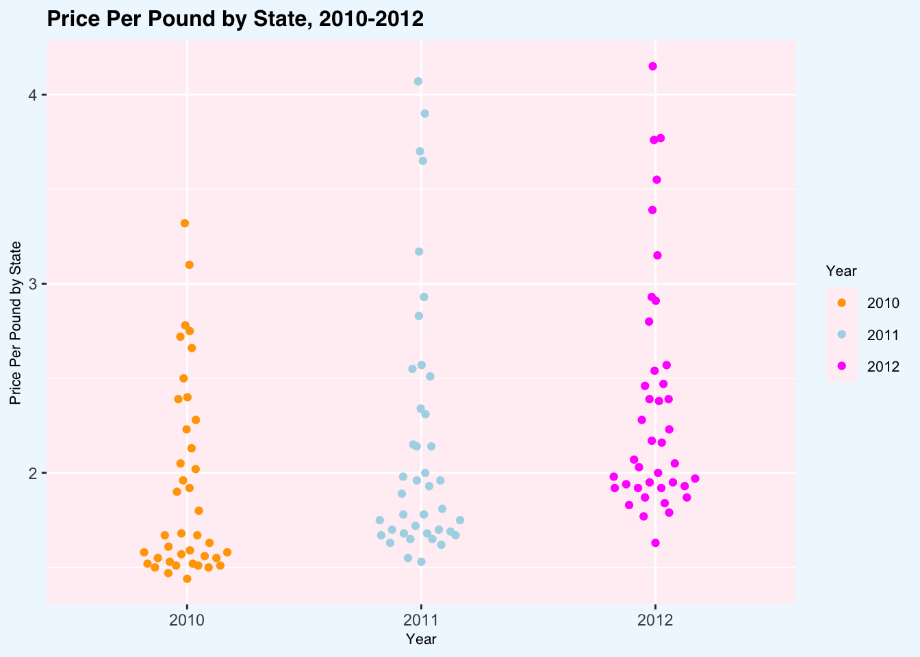

Plot 2

p2 <- ggplot(dataP2) +
  aes(x=yieldpercol, y=Cyear, fill=Cyear) +
  geom_density_ridges(
    aes(point_color = Cyear, 
        point_fill = Cyear, 
        point_shape = Cyear),
    alpha = .2, 
    point_alpha = 1, 
    jittered_points = TRUE) +
  scale_point_color_hue(l = 40) +
  scale_discrete_manual(aesthetics = "point_shape", 
                        values = c(21, 22, 23, 24, 25)) +
  labs(title = "Yield Per Colony Distribution by Year", 
       x = "Yield Per Colony", 
       y = "Year", 
       point_shape = "Year", 
       point_color = "Year", 
       point_fill = "Year", 
       fill = "Year") +
  theme(
    plot.title = element_text(family = "helvetica", face = "bold", size = 12),
    axis.title = element_text(family = "helvetica", size = 8),
    legend.title = element_text(size = 8), 
    legend.text = element_text(size = 8), 
    plot.background = element_rect(fill = "aliceblue", color = NA), 
    panel.background = element_rect(fill = "lavenderblush"),
    legend.background = element_rect(fill = "aliceblue")
  )
p2

## Warning: The `scale_name` argument of `discrete_scale()` is deprecated as of ggplot2
## 3.5.0.
## This warning is displayed once every 8 hours.
## Call `lifecycle::last_lifecycle_warnings()` to see where this warning was
## generated.

## Picking joint bandwidth of 6.44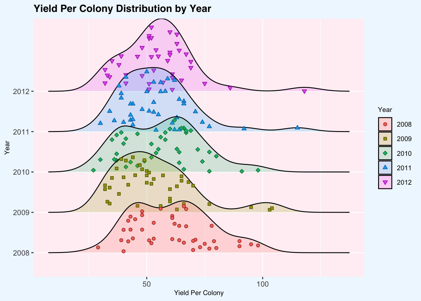

Plot 3

p3 <- ggplot(data) +
  aes(x=yieldpercol, y=priceperlb) +
  geom_bin2d(binwidth = c(3,0.10)) +
  scale_fill_gradientn(colors = c("pink", "magenta")) +
  labs(title = "Price Per Pound Based on Colony Yield", 
       x = "Yield per Colony", 
       y = "Price Per Pound") +
  theme(plot.title = element_text(family = "helvetica", face = "bold", size = 12),
        axis.title = element_text(family = "helvetica", size = 8),
        legend.title = element_text(size = 8), 
        legend.text = element_text(size = 8), 
        plot.background = element_rect(fill = "aliceblue", color = NA), 
        panel.background = element_rect(fill = "lavenderblush"),
        legend.background = element_rect(fill = "aliceblue"))
p3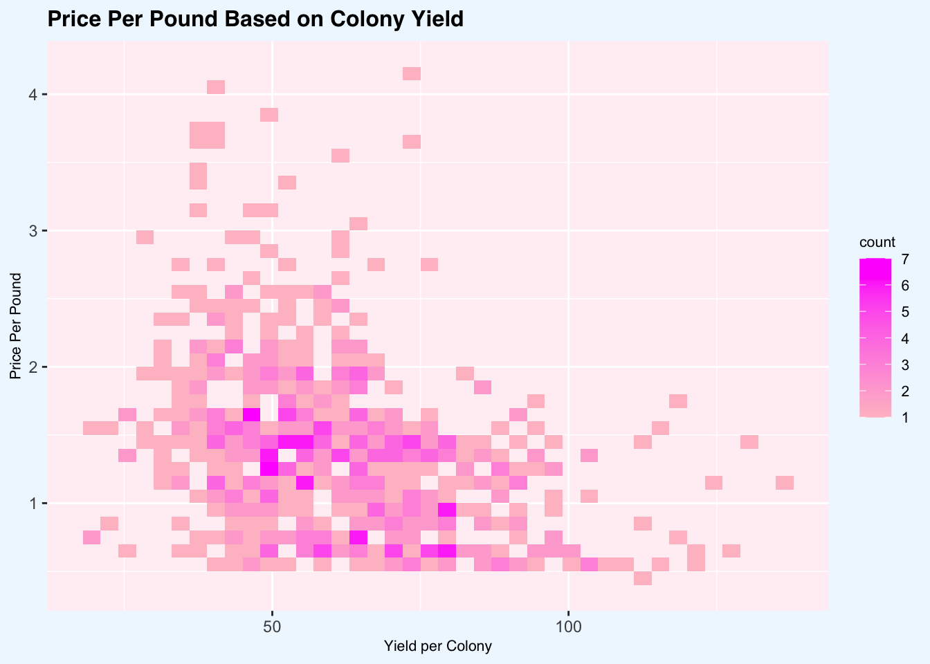

Plot 4

p4 <- ggplot(dataP4) +
  aes(x="", y=meanprod, fill=state) +
  geom_bar(stat="identity", width = 1, color = "white") +
  coord_polar("y", start=0) +
  geom_label_repel(
    aes(y = label_pos * sum(meanprod), label = label),
    x = 1.4,
    nudge_x = 0.5,
    show.legend = FALSE,
    size = 4,
    segment.color = "gray50"
  ) +
  scale_fill_brewer(palette = "Pastel1") +
  labs(title = "Mean Total Product of Great Plains States",
       fill = "State") +
  theme_void() +
  theme(plot.title = element_text(family = "helvetica", face = "bold", size = 12),
        legend.title = element_text(size = 8), 
        legend.text = element_text(size = 8), 
        plot.background = element_rect(fill = "aliceblue", color = NA), 
        panel.background = element_rect(fill = "lavenderblush"),
        legend.background = element_rect(fill = "aliceblue"))
p4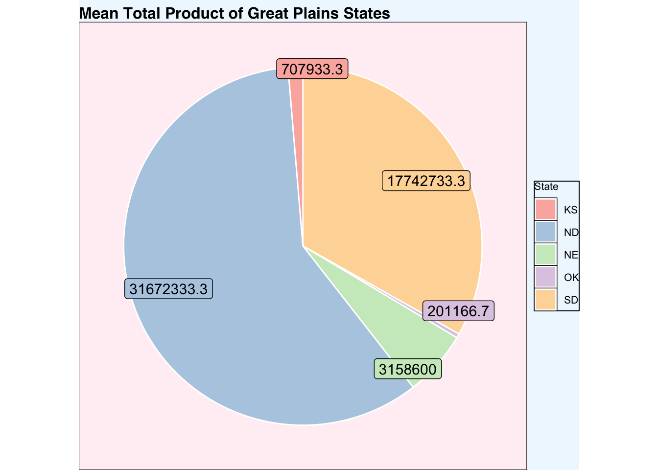

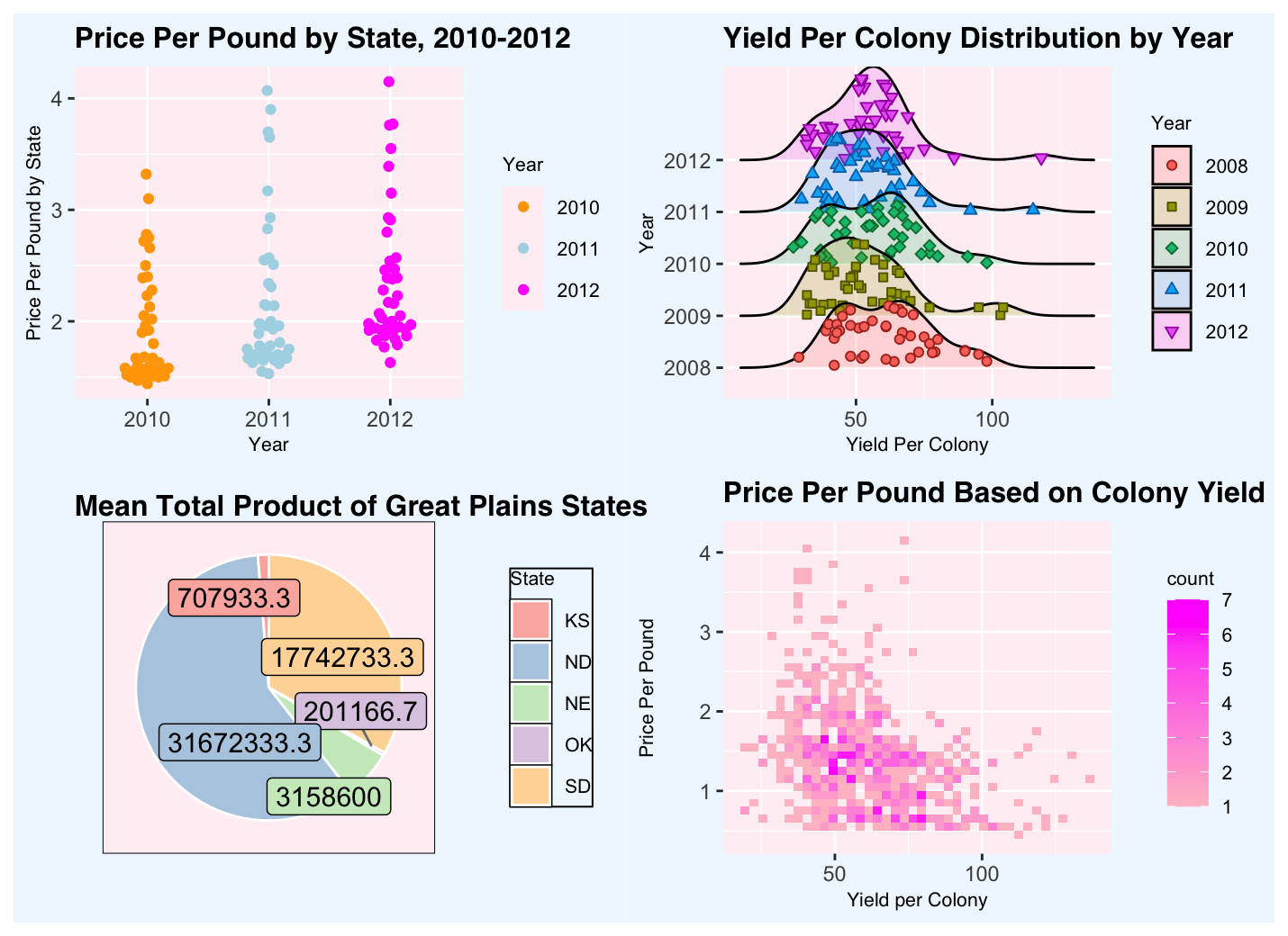
Cumulative Plot

p1 + p2 + p4 + p3 + plot_layout(ncol=2, widths = 1, heights = 1)

## Picking joint bandwidth of 6.44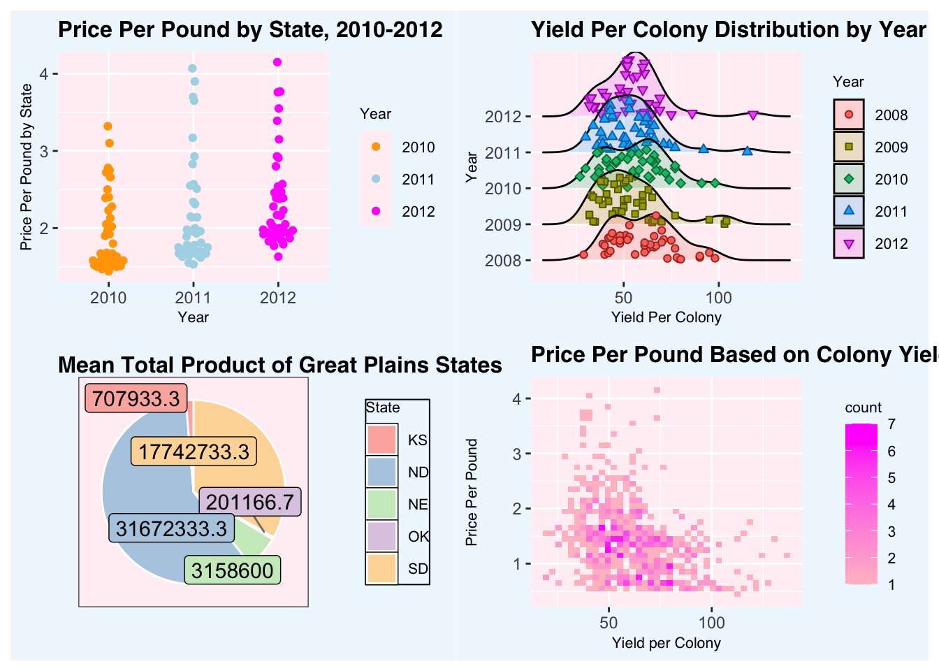

PNG: Cumulative Plot